How does AI work?

In the previous post in our series about AI, you can find a high-level introduction on how it works. This post goes a bit more technical, and by the end of it, you will know how simple AI models work in reality, and even run a model.
Building Simple AI Models
We will take a very simple example and slowly build up from there. The main aim of AI models is to generate output from an input that closely matches the expected result. We will explore how this process works in this post.
Layers in Machine Learning Models
Machine learning models are constructed of layers. Simpler models have fewer layers, but more complex models can have hundreds, and thousands of them. Every model has two essential layers: the input and the output layers. Deep learning models have hidden layers between them. For demonstration, our model will not have hidden layers, but the concept is similar regardless of the number of layers.
The Linear Function
It’s surprising to many people when they realize that the barebones of AI is a very simple mathematical function, the linear function (even ChatGPT is constructed upon it):
\[ ax + b = y \]
If we simplify it, a machine learning model is essentially arbitrary numbers, called weights (\( a \), and \( b \)). The weights multiplying the input \( x \) will return the output \( y \).
The goal of training a machine learning model is to find the correct weights (\( a \) and \( b \)) that result in the correct output \( y \) for the given input \( x \).
When we start training a model, the weights are randomised, so it's unlikely it will return the correct result.
But how will the weights be corrected?
Shooting range example
Imagine that you are on a shooting range. You are only able to move on the base line, and can turn up to 90 degrees either side. There are several melons scattered on the field, and your goal is to hit as many as you can with one shot. But there’s a twist: you’re blindfolded.
The only guide you are going to get is how far each target is from the baseline.
Without any further references, you take a random shot, and then you get the results - how far off your bullet was from each target.
If you notice that the closer targets to you were closer to the bullet than the further targets, you turn, and adjust your aim.
If the bullet's distance from each target is similar, you move along the baseline.
Eventually, after trial and error, and adjusting your position based on the results, you get closer and closer to the targets.
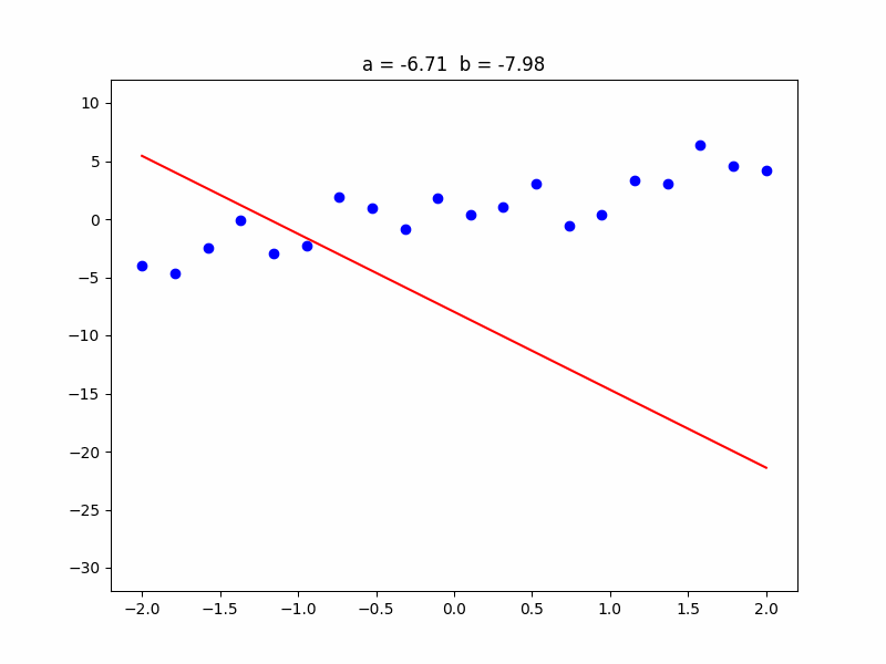
In the analogy, the way of the bullet is represented by the red (regression) line. The baseline is the \( y \) axis of the graph, along which you can move, adjusting the height \( b \) of the regression line. The angle of aim is the slope \( a \) of the regression line.
The input \( x \) is the distance of melons from the baseline (\( y \) axis), and the output \( y \) is the position of melons along the \( y \) axis.
Math
We are going to construct a very simple one node machine learning model that is a linear function solver.
To make it even simpler, we will eliminate \( b \) from the equation by assuming it’s 0, transforming the equation into:
\[ ax = y \]
Where \( a \) is the weight, \( x \) is the input, and \( y \) is the output.
As mentioned before, we start training a model, we randomise the weights. This is a crucial part of the training's success.
Example of Training
Let’s train a very simple model:
- Input 1 should output 2.
- Input 3 should output 6.
Let's annotate the desired output with \( o \).
It’s visible that we multiply the input \( x \) by 2 to get the desired outputs, but the model doesn’t know that yet. We start with random weights; let’s say \( a \) is 1.
First Training Step
In the first training step:
- Multiplying 1 with 1 results in 1, but it should be 2.
- Multiplying 3 by 1 results in 3, while it should be 6.
That’s where we evaluate the results and calculate the loss. The loss measures the error in the actual and expected result. There are multiple “loss functions”. We will use a simple one, called mean squared error, where we add up the differences between the desired output \( o \), and the predicted output \( y \) for both data points, square it to keep it positive, and divide it by the number of data points:
\[ \text{loss} = \frac{((2-1)^2 + (6-3)^2)}{2} = \frac{10}{2} = 5 \]
This is the loss, or cost.
Adjusting the Weights
The goal in training is to adjust the weights. We calculate how much influence the weight had in producing the result, relative to the loss (\( \frac{dC}{dw} \)).
Calculating the Gradient
To calculate this, we must determine each layer’s influence on the output, hence the loss. We reverse what we did to get the output, figuring out what should have been changed to get the ideal result. Technically, these are called gradients, and the process of reversing what we’ve done is called backpropagation.
We need to calculate:
- The influence of cost relative to the output (\( \frac{dC}{dy} \)).
- The influence of the output relative to the weight (\( \frac{dy}{dw} \)).
Calculating the Influence
The influence of cost relative to the output is the derivative of the mean squared error:
\[ \frac{dC}{dy} = -\frac{2}{2} * (y - o) \]
So \[ \frac{dC}{dy} = -((2 - 1) + (6 - 3)) = -4 \]
The influence of the output relative to the weight is simply the input, so \[ \frac{dy}{dw} = 1 + 3 = 4 \]
Thus, \[ \frac{dC}{dw} = \frac{dC}{dy} * \frac{dy}{dw} = -4 * 4 = -16 \]
This is called the gradient of the weight.
Adjusting the Weight
We multiply the learning rate (usually a small number like 0.01) with the gradient, and subtract it from the weight:
\[ w = 1 + 16 * 0.01 = 1.16 \]
This weight is much closer to the equilibrium that is 2. If the learning rate were higher, like 0.2, we would actually go further from the optimal weight, increasing to 4.2. That would result in what's called exploding gradient, where in each training step we would get worse training results.
Continual Adjustments
We keep making small adjustments on the weights until they reach the optimum and no longer improve. Imagine rolling a ball down from the edge of a round bowl. It rolls back and forth, with less momentum each time until it eventually stops at the bottom of the bowl. This behavior, where we adjust the weights to reduce the gradients, is called gradient descent.
In the next chapter, we will explain how this works on a larger scale.