AI in depth

We highly encourage you if you didn't yet to read the previous part, where we showed how the machine learning model performs the forward pass, predicting the output, calculating the loss by comparing the prediction with the actual result, and updating the weights to improve predictions.

We used a simple linear regression model and a few numbers to demonstrate the process. In reality, these models operate on a much larger scale using multi-dimensional matrices, but it's not as complex as it first appears.

Evaluating and Training Models at Scale

When we evaluate and train models at a large scale, instead of calculating the outputs based on inputs one by one, we use matrices for efficiency and clarity. During the forward pass, we input multiple data points in batches to process them simultaneously.

Inputs are usually not just single numbers, but consist of multiple features. In this post as example, we will use a dataset of real estate properties. At the end, based on the number of bedrooms and square footage, we will train a model to predict the property value and the expected time to sell.

Single Feature Model

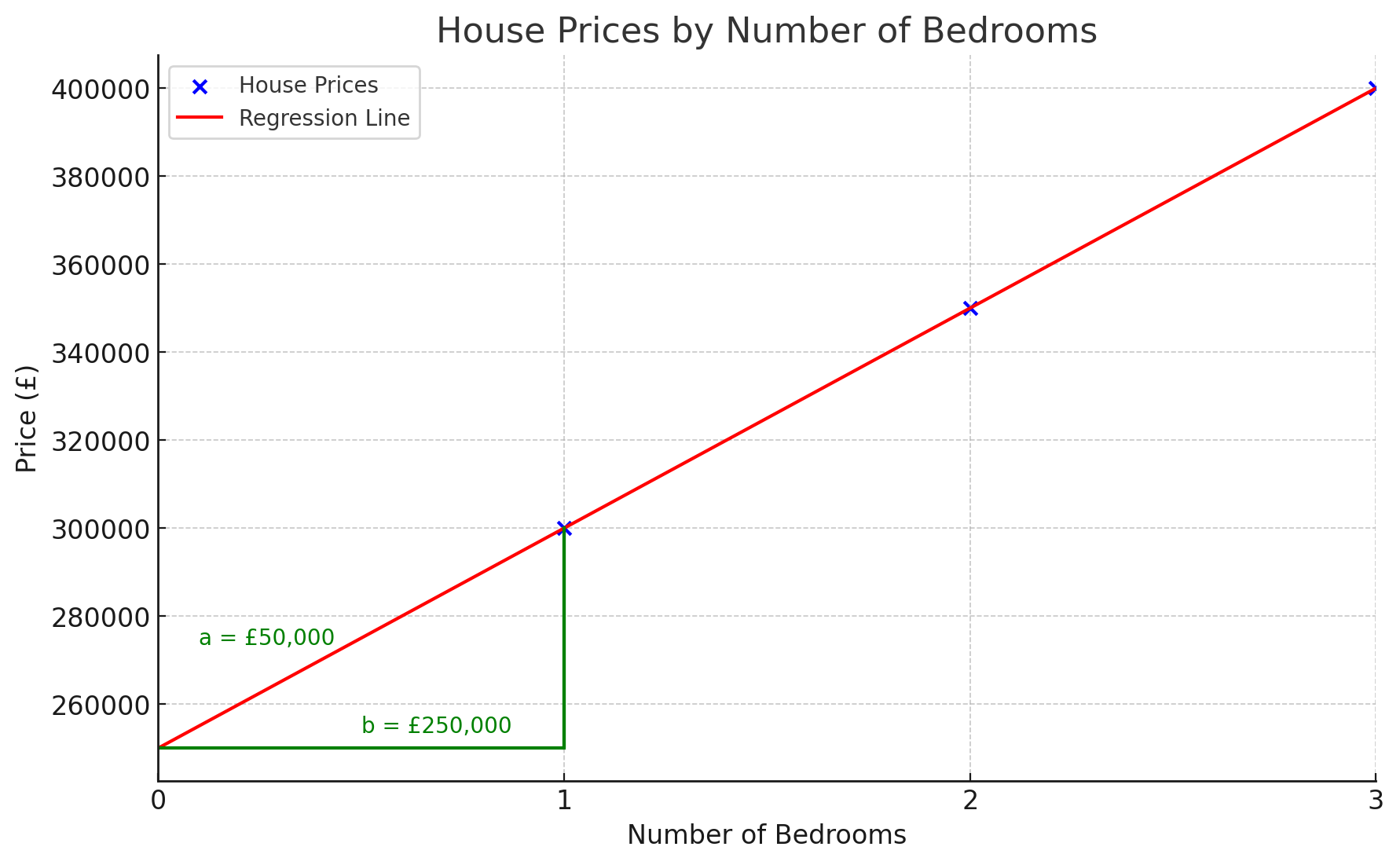
Let's start simple. The input will consist of one feature, the number of bedrooms, and the output will be the value of the property. This will be a single-dimensional model, as one input connects with one output.

• 1 bedroom: £300,000
• 2 bedrooms: £350,000
• 3 bedrooms: £400,000

So:

\(x_1 = 1, y_1 = 300000\)

\(x_2 = 2, y_2 = 350000\)

\(x_3 = 3, y_3 = 400000\)

With proper training, the model will eventually figure out that \( b = 250000 \) and \( a = 50000 \).

This simple example highlights two problems. First, writing down every number might be feasible for 3 data points, but AI is trained on millions. Second, the model is not very accurate. For example, a 3-bedroom house might cost £200,000 in one area but £1,000,000 in London. We need to add additional features to be able to get accurate results.

Using Matrices

Previously we used a single-node linear regression model to show the execution and training process. In reality, these models operate on a larger scale using multi-dimensional matrices, but it’s not as complex as it sounds.

Training data in a matrix would look like this:

A matrix has dimensions and shape.

• 0 dimensions: a single number like \( 4 \)
• 1 dimension: a list of numbers, \([10, 24, 32, 3]\) with shape \( [4] \)
• 2 dimensions: a table of numbers like the above with shape \( [3, 2] \), \[ \begin{bmatrix} 1 & 300000 \\ 2 & 350000 \\ 3 & 400000 \\ \end{bmatrix} \]

Matrix Multiplication

Instead of calculating each data point individually, we use matrices and perform linear function calculations simultaneously. This approach is faster and cleaner.

Single Data Point Example

Let’s see an example of how matrix multiplication works with a single data point.

To calculate the bias, we “pad” the inputs with 1, so it always results in the bias \( b \) itself.

If you notice, the calculation is still \( y = ax + b \), where \( x \) is the number of bedrooms.

Multiple Data Points Example

Now observe how it simplifies the process for multiple data points.

In matrix multiplication, we multiply each element in the rows of the first matrix with the columns of the second matrix, then sum them. The result appears at the intersecting cell of the column and row.

Two important rules of two-dimensional matrix multiplication:

• The number of columns in the first matrix must match the number of rows in the second matrix.
• The result matrix will have the same number of rows as the first matrix and the same number of columns as the second matrix.

Here’s an illustration of matrix multiplication for the multiple data points:

Adding Another Feature

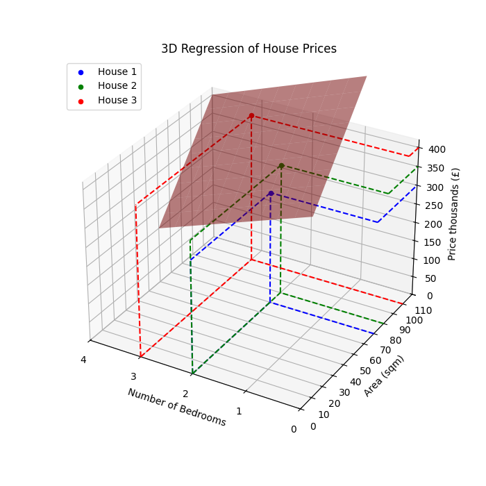
Now for the second issue - let’s imagine we are valuing properties in a specific area to avoid extreme price differences between houses with similar features. Still, even two neighbouring houses with the same number of bedrooms can have significant differences in price. One of the relatively reliable metrics in house valuation is price/area, so we are going to add area to the features.

We extended the model with an additional dimension. Our data points now cannot be visualised on a two-dimensional graph but three.

Here’s how it would look:

The number of columns in the first matrix must match the number of rows in the second matrix, so we add a new weight.

This changes the linear function to:

\( y = b + x_1 \cdot a_1 + x_2 \cdot a_2 \)

Here’s how it looks in matrix multiplication:

Adding a New Output Category

Instead of predicting only the property value, we will also predict the number of months expected to sell.

This changes our equations to:

\( y_{r,0} = b_{0} + x_{r,0} \cdot a_{1,0} + x_{r,1} \cdot a_{2,0} \)

\( y_{r,1} = b_{1} + x_{r,0} \cdot a_{1,1} + x_{r,1} \cdot a_{2,1} \)

Where \( r \) is a row (like House 1), and the first index next to each notation is the row index, the second is the column index. It will make much more sense later.

Although this may seem complex, in matrix multiplication, it is just a new column in our weights matrix:

Which is the same as training two models for the different outputs, it's just much more efficient in one model. Notice that the price weights don't have an influence on the months weights, and their results don't influence each other either.

If you recognise the pattern, we can have as many features and output categories as we like, which just adds new rows and columns to our matrices.

Benefits of Matrices

• Scalability: Regardless of the number of data points, features, or output dimensions, the model can handle millions or just one without changing its description.
• Computational benefits: AI is trained with GPUs, which are well-suited for working with matrices due to their ability to perform many tasks in parallel.

Training process

In the training process, where we calculate the loss and gradient, the principle is the same as running the model. Instead of working with single numbers, we use matrices, effectively “reversing” the operation.

Prediction

For better understanding, previously we referenced our data using their everyday names, but technical labeling makes the calculations simpler. From now on:

Inputs:

• \( x \) is the matrix of the input data points
• \( x_{r} \) is a row in the data points i.e. House 1
• \( x_{r,c} \) is a specific feature in a data point i.e. House 1's Bedrooms

Outputs:

• \( \hat{y} \) is the matrix of the output, or prediction of the model
• \( y \) is the label, the expected output specified in the training data
• \( y_{r} \) or \( \hat{y}_{r} \) is a row in the outputs i.e. House 1's outputs
• \( y_{r,c} \) or \( \hat{y}_{r,c} \) is a specific output of a data point i.e. House 1's Expected sale in months

Weights:

• \( w \) is the matrix of the weights - we don't distinguish \( b \) from \( a \) anymore
• \( w_{r} \) is a row in the weights, corresponding to a feature in the inputs i.e. weights of bedrooms
• \( w_{r,c} \) is a specific weight for a given feature, and output category i.e. the weight for calculating the house price based on the house's bedrooms

As we saw previously with the house example, to run the model, and make a prediction, it's matrix-multiplying the inputs with the weights: \( \hat{y} = x * w \)

Adjusting the weights

As we learnt in the previous post in the series, we basically reverse the prediction process, and try to find what should have been adjusted to reduce the cost - the difference between the prediction, and the expected output - using the chain rule:

\[ \frac{dC}{dw} = \frac{dC}{dy} * \frac{dy}{dw} \]

First, get \( \frac{dC}{dy} \) - how much influence did the prediction had on the cost - which is the derivative of mean squared error (we use the simplified version here, subtracting the expected output from the prediction).

Then, get \( \frac{dy}{dw} \) - which is the most straightforward as only the inputs \( x \) have influence on the weights to produce the predictions.

Finally, calculate \( \frac{dC}{dw} \) - we have to transpose (rotate 90 degrees in human language) the inputs to get the correct shape for the weights, and multiply by \( \frac{dC}{dy} \):

Now that we calculated the gradient (\( \frac{dC}{dw} \)), we just multiply it with the learning rate, and subtract it from the weights to get the new weights:

Conclusion

Matrices are very useful and efficient in machine learning, simplifying the process, and making it scalable - in an actual machine learning model code, when executing or training, adding new weights, it requires very little effort to add hundreds or thousands of new weights, or work with millions of data points.

Two useful tips:

Something to remember is while these illustrations are useful in the beginning to understand how fundamental principles of AI work, don't get hang up on trying to visalise them. In fact, this simple linear regression model is as far as we can go visualising in maximum 3 dimensions - more advanced models require us to think in \( n \) dimensions, which is not something we can visualise.

Most AI models are collection of millions weights that are usually pretty ugly numbers (like \( -0.0043570347 \)) distributed over n dimensions. This is why thinking in notations, and matrices is a lot cleaner.

Next Steps

In this section, we trained a linear regression machine learning model. In the next section, we will explore how a deep learning neural network functions.